What I Learned Modeling a Production Planning Problem with LP

Background

The first time I tackled a real-world supply chain planning problem, I struggled to calculate the right allocation of supply-constrained components to different products with overlapping bills of materials (BOM). Later, through MITx’s Supply Chain Management MicroMasters courses, I learned that linear programming was exactly the tool I needed. Here’s an example demonstrating what I wish I’d known back then.

Production planning example: what should we build to minimize cost?

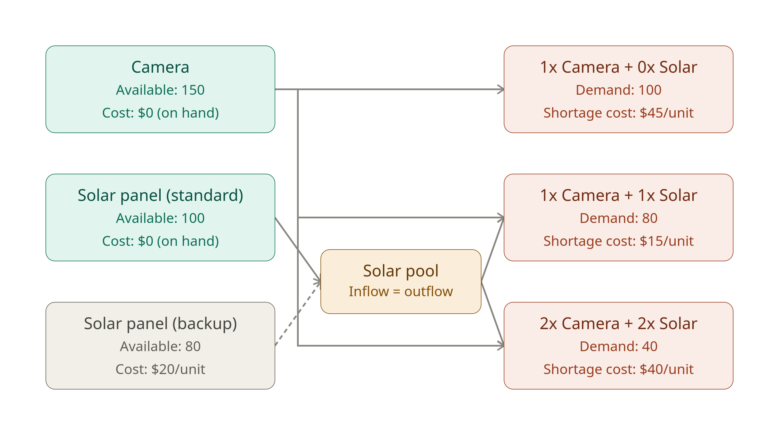
Problem statement

Given a fixed on-hand inventory of wire-free security cameras and standard solar panels, and access to a more expensive backup solar panel source, determine the production quantity for each of three product bundles that minimizes total cost — where cost consists of backup sourcing expenses plus a penalty for any unmet demand, with penalties varying by product.

Decision variables

• $q_1, q_2, q_3$ — units produced of Product 1 (1x camera + 0x solar), Product 2 (1x camera + 1x solar), and Product 3 (2x camera + 2x solar)
• $s_1, s_2, s_3$ — unmet demand (shortage) for Product 1, 2, and 3
• $u_{std}$ — units of solar panel sourced from standard (on-hand) inventory
• $u_{bu}$ — units of solar panel sourced from the backup supplier

Objective

\[\text{Minimize cost:} \quad 20\,u_{bu} + 45\,s_1 + 15\,s_2 + 40\,s_3\]

Constraints

Camera supply

\[q_1 + q_2 + 2q_3 \le 150\]

Solar panel pool (supply must equal demand)

\[q_2 + 2q_3 = u_{std} + u_{bu}\]

Solar sourcing limits

\[u_{std} \le 100, \qquad u_{bu} \le 80\]

Demand (with s absorbing shortage)

\[q_1 + s_1 = 100, \qquad q_2 + s_2 = 80, \qquad q_3 + s_3 = 40\]

Non-negativity

\[q_1, q_2, q_3, s_1, s_2, s_3, u_{std}, u_{bu} \ge 0\]

Sample Python solution

View Code Example

"""
Bundle allocation LP: minimize total cost (backup sourcing + unmet-demand
penalties) subject to camera supply, solar pooling, and demand constraints.

Requires: pip install pulp
"""

import pulp

# ---------------------------------------------------------------------
# Model
# ---------------------------------------------------------------------
model = pulp.LpProblem("bundle_allocation", pulp.LpMinimize)

# --- Decision variables -------------------------------------------------
# Production quantities
q1 = pulp.LpVariable("q1_1cam_0solar", lowBound=0)   # 1x camera + 0x solar
q2 = pulp.LpVariable("q2_1cam_1solar", lowBound=0)   # 1x camera + 1x solar
q3 = pulp.LpVariable("q3_2cam_2solar", lowBound=0)   # 2x camera + 2x solar

# Unmet demand (shortage variables)
s1 = pulp.LpVariable("s1_unmet_p1", lowBound=0)
s2 = pulp.LpVariable("s2_unmet_p2", lowBound=0)
s3 = pulp.LpVariable("s3_unmet_p3", lowBound=0)

# Solar sourcing
u_std = pulp.LpVariable("u_std_solar", lowBound=0)   # on-hand, free
u_bu = pulp.LpVariable("u_bu_solar", lowBound=0)     # backup, $20/unit

# --- Objective ------------------------------------------------------------
# Shortage costs: $45/unit (P1), $15/unit (P2), $40/unit (P3, raised from $30
# to break the tie with P2 on penalty-avoided-per-camera-unit)
model += (
    20 * u_bu
    + 45 * s1
    + 15 * s2
    + 40 * s3
), "total_cost"

# --- Constraints ------------------------------------------------------
model += q1 + q2 + 2 * q3 <= 150, "camera_supply"
model += q2 + 2 * q3 == u_std + u_bu, "solar_pool_balance"
model += u_std <= 100, "standard_solar_cap"
model += u_bu <= 80, "backup_solar_cap"
model += q1 + s1 == 100, "demand_p1"
model += q2 + s2 == 80, "demand_p2"
model += q3 + s3 == 40, "demand_p3"

# ---------------------------------------------------------------------
# Solve
# ---------------------------------------------------------------------
model.solve(pulp.PULP_CBC_CMD(msg=False))

print(f"Status: {pulp.LpStatus[model.status]}")
print(f"Total cost: ${pulp.value(model.objective):,.2f}\n")

print("Production plan:")
for var, label in [(q1, "P1 (1x cam + 0x solar)"), (q2, "P2 (1x cam + 1x solar)"), (q3, "P3 (2x cam + 2x solar)")]:
    print(f"  {label:28s} {var.value():6.1f} units")

print("\nUnmet demand:")
for var, label in [(s1, "P1"), (s2, "P2"), (s3, "P3")]:
    print(f"  {label:28s} {var.value():6.1f} units")

print("\nSolar sourcing:")
for var, label in [(u_std, "Standard (free)"), (u_bu, "Backup ($20/unit)")]:
    print(f"  {label:28s} {var.value():6.1f} units")

Interpreting the output

Output:

Status: Optimal
Total cost: $1,800.00

Production plan:
  P1 (1x cam + 0x solar)        100.0 units
  P2 (1x cam + 1x solar)          0.0 units
  P3 (2x cam + 2x solar)         25.0 units

Unmet demand:
  P1                              0.0 units
  P2                             80.0 units
  P3                             15.0 units

Solar panel usage:
  Standard (free)                50.0 units
  Backup ($20/unit)               0.0 units

$1800 is the lowest cost we can achieve under the current set of constraints. The camera supply is a binding constraint. All 150 cameras were consumed. Given a scarce shared resource, the solver effectively asked “which product gives the most avoided-penalty per camera consumed?” and answered:

• P1 (1x cam + 0x solar): \$45 shortage cost ÷ 1 camera = \$45/camera
• P3 (2x cam + 2x solar): \$40 shortage cost ÷ 2 cameras = \$20/camera
• P2 (1x cam + 1x solar): \$15 shortage cost ÷ 1 camera = \$15/camera

That flexibility in solar panel sourcing turned out to be irrelevant, because the constraint that actually bound the problem was cameras, not solar panels.

Maybe you’re thinking that we could have arrived at this conclusion without linear programming, and that’s true for a problem of this size. However, imagine if the problem involved a larger number of products and assemblies - that’s when linear programming truly shines.